Solving Tile Sliding Puzzles With Graph Searching Algorithms


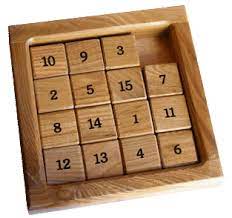
Puzzles are good way to kill some time when you're bored. I was at a doctors office the other morning, and in the waiting room they had sliding tile puzzle that I played around with for a little bit while waiting to be called in. Personally, I find writing algorithms to solve the puzzles for me to be an even better way to kill some time. A number of small tabletop puzzle games, like peg solitaire and various tile sliding games can be modeled algorithmically to find solutions to them. So when I got home, that's exactly what I did.
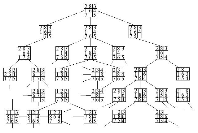
This can be generalized by viewing A puzzles configuration as it's state, with each possible new configuration resulting from moving a piece from the current configuration representing a state change. If we have an initial state, and our goal is to get to a finishing state, we can enumerate the possible state changes to create a tree structure that if possible, will guide us from a starting state to our goal state by traversing the tree. I've covered one approach to this technique, called backtracking, when discussing the N Queens problem. In this post I will be discussing the 8-sliding tile puzzle and various algorithmic techniques used for solving them.
First, lets cover some basics of sliding tile puzzles.
Understanding the Problem Space
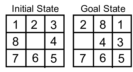
Sliding tile problems are based on a matrix of NxN spaces, with one blank space and the rest numbered 1 - N. Common values for N are 3, resulting in the 8-puzzle, and 4 which results in the 15 puzzle. The goal of the puzzle is to get from a starting configuration to a goal configuration by moving the rearranging the tiles using only allowable moves.
Before we can even think about solving these puzzles, it is important to know if a given starting configuration is even possible to solve - not all of them are. Thankfully, there is an easy way of determining this.
Determining If A Puzzle Can Be Solved
In the tabletop version of slider puzzles, the goal state is reached when the tiles are arranged numerically in row wise order. It should be noted that this technique is only applicable to puzzles whos final state is as pictured.
To determine if a puzzle can be solved depends on the size of the puzzle being solved. We begin by counting the inversions in the starting configuration. An inversion is when two numbers, 'A' and 'B' appear in the matrix, with the value of 'A' being greater than 'B' but appearing before it in the total ordering. In an NxN matrix, we count the number of inversions, again in row wise order.
If N is an odd number, then only puzzles with an even number of inversions can be solved.
If N is an even number, the puzzle can be solved only when the number of inversions + the row index of the blank space is even.
There are a number of ways to obtain the count of inversions, but all of them will involve flattening the matrix to a 1d Array. The following is the simplest approach, but keep in mind that it is n^2 complexity:
bool checkBoardIsSolvable(Board b) {
        vector<int> ordered;
        //flatten the 2d vector.
        for (auto row : b)
            for (auto col : row)
                ordered.push_back(col);
        //count inversions
        int inversions = 0;
        for (int i = 0; i < 8; i++) {
            for (int j = i+1; j < 9; j++) {
                //The blank space is not used in the inversion count
                if (ordered[i] && ordered[j] && ordered[i] > ordered[j])
                    inversions++;
            }
        }
        //odd size puzzle, must have an even number of inversions.
        if (b[0].size() % 2 != 0 && inversions % 2 == 0)
            return true;
       //even size puzzle, add the row index of the blank spot
        if (b[0].size() % 2 == 0 && (inversions + (find(b, 0).y+1)) % 2 ==0)
            return true;
        return false;
    }
Another method of counting inversions is simply to merge sort the flattened array, and track the inversions it encounters during the sort. If you are not using a flattened array, but instead using a 1d representation of the board, then remember to sort a copy of the board, not the original. This reduces the complexity to O(n log n):
int countInversions(vector<int>& a, vector<int>& aux, int l, int r, int inv) {
    if (r - l <= 1)
        return inv;
    int m = (l+r) / 2;
    inv = countInversions(a, aux, l, m, inv);
    inv = countInversions(a, aux, m, r, inv);

    for (int k = l; k < r; k++) aux[k] = a[k];
    int i = l, j = m, k = l;
    while (i < m  && j < r) {
        if (aux[i] < aux[j]) {
            a[k++] = aux[i++];
        } else {
            //inversion!
            a[k++] = aux[j++];
            if (aux[i] && aux[j-1])
                inv++;
        }
    }
    while (i < m) a[k++] = aux[i++];
    while (j < r) a[k++] = aux[j++];
    return inv;
}

bool checkBoardIsSolvable(Board b) {
   vector<int> ordered;
   for (auto row : b)
      for (auto col : row)
          ordered.push_back(col);
   vector<int> aux;
   aux.reserve(ordered.size());
   int inversions = countInversions(ordered,aux, 0, ordered.size(), 0);
   if (b[0].size() % 2 != 0 && inversions % 2 == 0)
            return true;
   if (b[0].size() % 2 == 0 && (inversions + (find(b, 0).y+1)) % 2 ==0)
            return true;
        return false;
 }
To be honest, these puzzles are generally small enough that the brute force method of counting inversions perfectly sufficient. I've included the merge sort based method for the sake of completeness.
Proceeding When A Puzzle is Solvable
Once we've determined that a puzzle is able to solved, we proceed by trying different board configurations. The board can be reconfigured by swapping the blank space with any of its neighbors immediately above, below, to the left, or to the right of it. Spaces can not be swapped horizontally however. Seeing as each board can potentially have up to 4 possible next states, the search space can be quite large due to combinatorial explosion. Knowing this, we can assume that any technique that reduces the size of the search space can aid in speeding up the search.
There are two basic techniques for approaching searching problems. Informed search is applicable when we can exploit some known properties of the puzzle to aid us in making a better decision when selecting which state to transition to next. An example of this being A* search.
The other approach is what's called "uniformed search". That's a fancy way of saying brute force, where we treat any next state as equally likely and traverse them all, albeit in different orders depending on the method chosen. Depth First Search and Breadth First Search are two such examples of this approach - and being the simplest types of search, they make a good place to start.
Laying the Foundation
Despite there being a number of different ways to proceed all of them require a few things in common:
- Need a practical way of representing the board in memory
- Must have a procedure to generate the possible next states of a given board
- Some way to represent the relationship between states
- And a method to compare a given board to the goal state.
With the board being a simple matrix, it is only logical for it to be represented by a 2d array of integers. I used the C++ vector class because it allows us to avoid some of the boilerplate involved in constructing the matrix.
For representing the relationship between different board states, we are going to use a special kind of tree structure called a state space tree. Each possible next state makes up the children nodes of the current board state in our tree. I chose to use a Left Child/Right Sibling tree with an additional parent pointer (to aid in retracing solution paths) as the data structure. Each node of the tree has a copy of the board, the x/y coordinates of the blank spot in the matrix, a pointer to its first child node, as well as a pointer it's sibling nodes.
typedef vector<vector<int>> Board;

struct point {
    int x, y;
    point(int X = 0, int Y = 0) {
        x = X; y = Y;
    }
};

struct node {
    Board board;
    point blank;
    node* parent;
    node* next;
    node* children;
    node(Board info, point blank, node* parent, node* next) {
            this->blank.x = blank.x;
            this->blank.y = blank.y;
            this->board = info;
            this->next = next;
            this->parent = parent;
            this->children = nullptr;
    }
};

typedef node* link;
To generate the child nodes of a board, we pass the current node to a function that uses an array of coordinate off sets that will be applied to the coordinates where blank tile is located to aid in generating the next state. After applying the offsets to the blank spots coordinates, we check if the new coordinates are a valid board position, and if so swap those positions and create a child node for that state.
vector<point> dirs = {{1, 0}, {-1, 0}, {0,1},{0,-1}};
int tryCount = 0;

bool isSafe(int x, int y) {
     return x >= 0 && x < 3 && y >= 0 && y < 3;
}

link generateChildren(link h) {
        for (point d : dirs) {
            point next = {h->blank.x+d.x, h->blank.y+d.y};
            if (isSafe(next.x, next.y)) {
               Board board = h->board;
               swap(board[next.x][next.y], board[h->blank.x][h->blank.y]);
               h->children = new node(board, next, h, h->children);
               tryCount++;
           }
       }
       return h->children;
}
The child state nodes are linked together in a linked list, with each child node also pointing back to its parent. To know if we've found a solution we need an equality check for our boards, as well as way to display the boards.
 bool compareBoards(Board a, Board b) {
     for (int i = 0; i < 3; i++)
        for (int j = 0; j < 3; j++)
           if (a[i][j] != b[i][j])
              return false;
    return true;
}

void printBoard(Board& board) {
     for (vector<int> row : board) {
         for (int col : row) {
            cout<<col<<" ";
         }
         cout<<endl;
     }
}
And of course, we're going to need a driver program to test our algorithms, the following is what I used:
 int main() {
   Board p1start = {
                   {2,8,3},
                   {1,6,4},
                   {7,0,5}
                 };

    Board p1goal = {
                   {1,2,3},
                   {8,0,4},
                   {7,6,5}
                 };

    Board p2start = {
                    {1, 2, 3},
                    {5, 6, 0},
                    {7, 8, 4}
                    };

    Board p2goal = {
                    {1, 2, 3},
                    {5, 8, 6},
                    {0, 7, 4}
                   };
    SlidePuzzle ep;
    ep.solve(p1start, p1goal);
    ep.solve(p2start, p2goal);
    return 0;
}
With these data structures and utility functions in place we are ready to start implementing a strategy to solve the puzzle, as mentioned above we will start with uninformed searches.
Exploring the Search Space
Our search space is organized as a tree, and with trees being a special type of directed acyclic graphs the logical place to start is with a graph searching algorithm. In general tree search algorithms work like this:
procedure search(start, goal):
        add start node to stack
        while (stack is not empty) {
            pop top item from stack and make current
            if (current is goal) {
                 show path from start to goal and exit.
            } else {
                 foreach (current.children)
                    add child to stack;
            }
        }
Some search techniques use recursion, and others are iterative. Some use a stack to store the nodes, and some use a queue while still others utilize a priority queue. Regardless of the exact strategy chosen, all tree searches work fairly similarly with some doing additional work to aid in the search.
Uninformed Searches
The simplest place to start is a recursive depth first search, so that is exactly what I did. I very quickly confirmed my suspicions that when you combine the size of each node with the combinatorial explosion of the search space, a depth first search will cause a stack overflow or run out of memory long before it finds a solution.
This happens because of the very nature of how depth first search works. Even if the goal state is located very close to the starting state in the tree but along a different branch then the one being traversed by DFS, it may not be reached. This means that even if we didn't smash the call stack with the depth of recursion or run out of memory from generating such a large tree, it could still take a VERY long time to arrive at the goal state - if it ever does at all.
One possible way to make depth first search avoid this type behavior is by imposing a limit on how far down a path we want to let it go before calling it quits and trying a different branch. This is called Depth Limited Search, and it requires only a one small change to DFS, the depth limit:
 void DLDFS(link curr, Board goal, int depth) {
        if (depth >= 0) {
            int cost = getBoardCost(curr->board, goal);
            if (cost == 0) {
                cout<<"Solution Found!\n";
                showSolution(curr);
                found = true;
                return;
            }
            if (curr->children == nullptr)
                curr->children = generateChildren(curr);
            for (link t = curr->children; t != nullptr; t = t->next) {
                if (!found)
                    DLDFS(t, goal, depth-1);
            }
        }
    }
Allright, lets see if we can find a solution within 8 moves:
max@MaxGorenLaptop:/mnt/c/Users/mgoren$ ./iddfs
 Trying with Depth Limit: 6
 Solution Found!
 1 2 3
 8 0 4
 7 6 5
------
 1 2 3
 0 8 4
 7 6 5
------
 0 2 3
 1 8
 7 6 5
------
 2 0 3
 1 8 4
 7 6 5
------
 2 8 3
 1 0 4
 7 6 5
------
 2 8 3
 1 6 4
 7 0 5
 Puzzle completed in 6 moves after trying 1800 board configurations.
 max@MaxGorenLaptop:/mnt/c/Users/mgoren$
Ok, now we're getting somewhere. But its not very convenient having to try and guess how many moves it should take - guess to high, and our search may not complete, guess to low and we may not find the solution. One possible remedy for this could be to use a variant of depth limited search called Iterative Deepening Depth First Search(IDDFS). IDDFS works just like depth limited search by monitoring how far down its current path the algorithm has progressed, and imposing a limit on it. When that limit is reached, the algorithm is forced to back track and try a different branch. Iterative deepening enhances this by repeatedly re-trying the search with increasing depth limits.
 bool found;
    void DLDFS(link curr, Board goal, int depth) {
        if (depth >= 0) {
            if (compareBoards(curr->board, goal)) {
                cout<<"Solution Found!\n";
                showSolution(curr);
                found = true;
                return;
            }
            if (curr->children == nullptr)
               curr->children = generateChildren(curr);
            for (link t = curr->children; t != nullptr; t = t->next) {
                if (!found)
                    DLDFS(t, goal, depth-1);
            }
        }
    }
    void iddfs(Board first, Board goal) {
        found = false;
        tryCount = 0;
        int last = 0;
        link start = new node(first, find(first, 0), nullptr, nullptr);
        for (int i = 2; i < 20; i++) {
            if (!found) {
                cout<<"Trying with Depth Limit: "<<i<<"\n";
                DLDFS(start, goal, i);
                cout<<"Search expanded "<<(tryCount-last)<<" nodes with no solutions found.\n";
                last = tryCount;
            } else {
                break;
            }
        }
        cleanUp(start);
    }
Ok, lets see where we get with IDDFS taking the guess work out of the depth limit for us:
max@MaxGorenLaptop:/mnt/c/Users/mgoren$ ./iddfs
 Trying with Depth Limit: 2
 Tried: 35 board configurations with no solution found.
 Trying with Depth Limit: 3
 Tried: 347 board configurations with no solution found.
 Trying with Depth Limit: 4
 Tried: 3499 board configurations with no solution found.
 Trying with Depth Limit: 5
 Solution Found!
 1 2 3
 8 0 4
 7 6 5
------
 1 2 3
 0 8 4
 7 6 5
------
 0 2 3
 1 8 4
 7 6 5
------
 2 0 3
 1 8 4
 7 6 5
------
 2 8 3
 1 0 4
 7 6 5
------
 2 8 3
 1 6 4
 7 0 5
------
 Puzzle completed in 6 moves after trying 683 board configurations.
 max@MaxGorenLaptop:/mnt/c/Users/mgoren$
All right! Success. Now, our search finds a solution after expanding 683 nodes. I would say a 1/3 reduction in the configurations needed to find a solution is definitely an improvement. IDDFS succeeds where regular DFS failed, because the depth limiting forces it to search a wider selection of branches than it normally would, in a way this is similar to how a breadth first search would perform. And just like Breadth First Search, IDDFS also has the desirable trait of finding a solution in the shortest number of moves possible.
Breadth First Search utilizes a First In First Out queue to explore each of a nodes children in turn before then searching their children, as opposed to depth first search which continues expanding the first child node it encounters due to its utilizing a Last In First Out ordered stack.
void BFS(link start, Board goal) {
     queue<link> fq;
     fq.push(start);
     while (!fq.empty()) {
         link h = fq.front();
         fq.pop();
         if (compareBoards(h->board, goal)) {
             cout<<"Solution Found!\n";
             showSolution(h);
             return;
         }
         h->children = generateChildren(h);
         for (link t = h->children; t != nullptr; t = t->next)
             fq.push(t);
     }
}
Breadth first search is not only simple to implement but it is also considered complete search wise, meaning that it is guaranteed to find the solution if one exists. So let's see how it does:
max@MaxGorenLaptop:/mnt/c/Users/mgoren$ ./8puzzle
 Solution Found!
 1 2 3
 8 0 4
 7 6 5
 -----
 1 2 3
 0 8 4
 7 6 5
 -----
 0 2 3
 1 8 4
 7 6 5
 -----
 2 0 3
 1 8 4
 7 6 5
 -----
 2 8 3
 1 0 4
 7 6 5
 -----
 2 8 3
 1 6 4
 7 0 5
 -----
 Puzzle completed in 6 moves after trying 683 board configurations.
max@MaxGorenLaptop:/mnt/c/Users/mgoren$
Hmm. Interesting result, It would seem that BFS expands the same amount of nodes as IDDFS, but this actually not *quite* the case. Every Node that BFS encounters it only ever explores once. Because of how IDDFS works, it repeatedly explores nodes that occur higher up in the tree. Looking at our example IDDFS found a solution at depth limit five, that means that every node in the first 4 levels of the tree were visited 5 times where BFS only visited them once. Even though we can thankfully skip the step of generating a nodes children after the first encounter, that's still a lot less work because of the drastic reduction in pointer surfing required, not to mention that BFS does not require recursion.
When is 'Good' good enough?
Lets take a moment to recap what we have accomplished up to this point. We've already gone from expanding so many nodes that our program would crash when using plain depth first search, to finding a solution after searching 683 nodes by employing a slight tweak to the algorithm. Now finding a solution after 683 tries with even less work and all it really took was a change in data structure. We could end here, having arrived at working solution for the 8-puzzle problem in the shortest amount of moves. But what if like for IDDFS & Depth First Search, we could see a huge improvement in performance for only a little more effort?
Looking back at our progress we can surmise that practically all of our improvements came about after making a fundamental change to the order in which the nodes were expanded. There is nothing similar to the DFS -> IDDFS trick that can be applied to Breadth First Search, but what we can do is swap out the FIFO queue for something a bit more powerful.
It is well known from graph algorithms that using a priority queue can lead to faster graph searching algorithms than BFS or DFS can provide, and our state space tree is really just a directed acyclic graph. But in order to use a priority queue we need to gather more information about the board state than we have been up to now, pushing us into the category of informed searches.
Informed Search
As I mentioned, for a priority queue to actually be useful, we need a way of assigning a distinct value to each state configuration. To assign this value, we will use the approximate distance from our current state to the goal state. We do this by summing the manhattan distance of each tile position in the goal state from where that value occurs in the current state.
If this sounds like it requires a lot more work, it's because it does. We are making a trade here. We are accepting a higher computational complexity cost for a (hopefully) drastic reduction in memory usage. In state space tree searching algorithms memory usage is directionally proportional to how many nodes of the tree need to be expanded in order to reach the goal.
In other words, while comparing the two board states will be a more computationally expensive operation than it would be for the previous algorithms, we will be doing it significantly less times because of how many fewer nodes we need to expand to find the solution.
point find(Board board, int x) {
        for (int i = 0; i < 3; i++) {
            for (int j= 0; j < 3; j++) {
                if (x == board[i][j])
                    return point(i, j);
            }
        }
        return point(-1,-1);
    }

    int getBoardCost(Board a, Board b) {
        int cost = 0;
        for (int i = 0; i < 3; i++) {
            for (int j = 0; j < 3; j++) {
                if (a[i][j] != b[i][j]) {
                   point p = find(b, a[i][j]);
                   cost += std::abs(i - p.x) + std::abs(j - p.y);
                }
            }
        }
        return cost;
    }
The getBoardBost() function replaces our previous implementation of compareBoards() that returned a bool. getBoardCost() will return 0 if the boards are the same, rendering compareBoards() redundant.
We will also use the value it returns as the cost for our priority queue. The lower the board cost, the closer to the goal state we are. By using a min-heap priority queue, we can keep selecting the closest next state instead of just trying them all as we did with BFS. This "greedy" method should significantly trim the search space and thus speeding up our search.
    typedef pair<int,link> pNode;
    void priorityFirstSearch(Board first, Board goal) {
        link start = new node(first, find(first, 0), nullptr, nullptr);
        priority_queue<pNode, vector<pNode>, greater<pNode>> pq;
        pq.push(make_pair(0, start));
        while (!pq.empty()) {
            link curr = pq.top().second;
            pq.pop();
            if (getBoardCost(curr->board, goal) == 0) {
                cout<<"Solution Found!\n";
                showSolution(curr);
                break;
            }
            curr->children = generateChildren(curr);
            for (link t = curr->children; t != nullptr; t = t->next)
                pq.push(make_pair(calculateBoardCost(t->board, goal), t));
        }
    }
As you can see, the algorithms are actually very similar with the main difference being the choice of data structure and the other changes being in the helper utilities to make use of the different data structure.
Lets run this version on the same puzzle we used for BFS and see if we gained any increase in performance:
max@MaxGorenLaptop:/mnt/c/Users/mgoren$ ./TilePuzzle
 Solution Found!
 1 2 3
 8 0 4
 7 6 5
------
 1 2 3
 0 8 4
 7 6 5
------
 0 2 3
 1 8 4
 7 6 5
------
 2 0 3
 1 8 4
 7 6 5
------
 2 8 3
 1 0 4
 7 6 5
------
 2 8 3
 1 6 4
 7 0 5
 Puzzle completed in 6 moves after trying 19 board configurations.
 max@MaxGorenLaptop:/mnt/c/Users/mgoren$
Wow! THAT is progress. We went from having to generate 683 different board configurations down to only 19 before we found our solution! Sure - each try cost more than it did for BFS, but the amount we chop from the search space more than makes up for that additional cost.
Additional Optimizations
During the course of this post I've covered focused primarily on the order nodes were visited, mainly by tweaking the data structure in an effort to complete the search while expanding as few nodes as possible.
Another optimization comes about due to the way our boards are generated. We run the risk of arriving back at a board that we have already visited - this is what is called a cycle in graph theory. And the above implementations do nothing to check for this case. In the worst case, a cycle could cause us to get stuck in an endless loop, with the BEST case being that we process more nodes than need be due to some being processed more than once. Thankfully we don't have to check each new configuration against every node already in the tree: we only need to compare it to the nodes along the path from the root to the current node, having maintained parent pointers makes this a very easy thing to do:
 bool hasSeen(link h) {
        if (h == nullptr || h->parent == nullptr)
            return false;
        node* x = h->parent;
        while (x != nullptr) {
            if (compareBoards(x->board, h->board)) {
                return true;
            }
            x = x->parent;
        }
        return false;
 }
And now we just need to check hasSeen(child) before deciding to expand the node, if it returns true we can skip expanding that node. Let's see how we do adding it to our PFS:
max@MaxGorenLaptop:/mnt/c/Users/mgoren$ ./pfs
Solution Found!
 1 2 3
 8 0 4
 7 6 5
------
 1 2 3
 0 8 4
 7 6 5
------
 0 2 3
 1 8 4
 7 6 5
------
 2 0 3
 1 8 4
 7 6 5
------
 2 8 3
 1 0 4
 7 6 5
------
 2 8 3
 1 6 4
 7 0 5
 Puzzle completed in 6 moves after trying 11 board configurations.
 max@MaxGorenLaptop:/mnt/c/Users/mgoren$
Well golly, It would appear we've chopped the search space nearly in half yet again! It is this checking of previously visited states that transforms our priority first search into the venerable A* search.
I think for now, this is far as I'm going to take things, seeing as in the course of this article, we've gone from polynomial to linear complexity on the 8-puzzle. Additionally, this optimization is also what tipped the scales and allowed it solve instances of the 15 puzzle, something it previously struggled to do (with some light tweaks to the heuristic).
max@MaxGorenLaptop:/mnt/c/Users/mgoren$ ./astar
 Solution Found!
 1 2 3 4
 5 6 7 8
 9 10 11 12
 13 14 15 0
---------
<removed for brevity>
---------
 1 6 2 7
 0 5 4 11
 10 15 14 3
 9 13 12 8
 Puzzle completed in 26 moves after trying 75 board configurations.
 max@MaxGorenLaptop:/mnt/c/Users/mgoren$
One simple optimization that led to a much better search, was to track what depth in the tree the current child is and store that in the node. When pushing a node to the priority queue, add the nodes depth to the priority.
That being said, some puzzles take ALOT more searching than others:
 max@MaxGorenLaptop:/mnt/c/Users/mgoren$ ./astar
 Solution Found!
 1 2 3 4
 5 6 7 8
 9 10 11 12
 13 14 15 0
---------
<removed for brevity>
----------
 15 14 1 6
 9 11 4 12
 0 10 7 3
 13 8 5 2
 Puzzle completed in 55 moves after trying 23997166 board configurations.
 max@MaxGorenLaptop:/mnt/c/Users/mgoren$
Still, Not bad for a couple hours of hacking.
Other Algorithms
There are other algorithms that can speed up the search even more, such as the many A* search variants. For puzzles with larger search spaces such as the 15-puzzle variant which uses a 4x4 matrix and the 24-puzzle which uses a 5x5 matrix, anything less than A* search isn't going to cut it. Iterative Deepening A* is considered the gold star for tile sliding puzzles - However, the algorithm is complicated enough that it really deserves it's own article.
Like A* search, the priority first search that was implemented above uses the cost function in a similar way to how A* uses heuristics. I only explored one heuristic in this post - there are many. Other cost functions/heuristics, so long as they are admissible have the potential to eek out even more performance from both algorithms. A* is a tricky beast however, It is only as good as heuristic. It may for example, return a 53 move solution when there is valid 48 move solution for example. BFS and IDDFS wont have this problem, but they also aren't up to the task of finding ANY solution for many 15 - puzzles.
An improvement upon breadth first search is a technique called Branch and Bound. Branch and bound works like the BFS counterpart to Backtracking DFS in that it utilizes a promising function to determine if a path is worth following. I encountered several websites through the course of my research that claim to be using branch and bound to solve sliding tile puzzles but are actually using best first search upon examination of the code.
Of perhaps a bit more interest, is that because we have a known goal state from the start, this problem is a feasible candidate for a bi-directional breadth first search, maybe even a parallel version with different threads searching from different directions - though I think we can all agree that might be just a touch overkill for a problem such as this.
There are also algorithms for solving these puzzles that require no searching at all - though they do not necessarily find the solution with least number of moves as the algorithms explained above do.
A Few Words About the Data Structures Used
The node structure that I implemented is admittedly overkill for the problem at hand. The reason I decided to construct a full LCRS representation of the state space tree is simply that I had never had occasion to ever use an LCRS tree before! Up to now they've just been something I've read about in DSA text books. My first implementation of the BFS algorithm shown above did not utilize child or parent pointers in the node structure. The tree was generated implicitly, with the children being a simple linked list, the solution path stored in a hash table. I find the implementation shown above to be far more elegant.
I also have an implementation that utilizes a quad tree available on my github page as linked below.
That's all I've got for you this today so until next time, Happy Hacking!
Further Reading
https://github.com/maxgoren/TilePuzzle
"Algorithms in a nutshell - a desktop quick reference" By Heineman, Pollice, & Selkow from O'reilly publishers.
"Data Structures Using C" By Tenenbaum, Langsam, & Augenstein
-
Fast Multi-Pattern String Searching with the Aho-Corasick Algorithm
-
Capture Groups: Tracking Regular Expression Sub Matches
-
Resolving Shift/Reduce Conflicts With Operator Precedence
-
Squeezing DFAs with Pair Compression
-
Designing Abstract Syntax Trees: Homogenous vs. Heterogenous Node Structures
-
From LR Items to LR States
-
Calculating Follow Sets of a Context Free Grammar
-
Streaming Images from ESP32-CAM for viewing on a CYD-esp32
-
Constructing the Firsts Set of a Context Free Grammar
-
Inchworm Evaluation, Or Evaluating Prefix-Expressions with a Queue
Leave A Comment