
Grids & Graphs
Grids are a special cases of Graphs called Lattice Graphs, and they show up and time and time again, particularly in Game Development. Certain categories of games, such as Rogue like games are heavily grid based.
For the purposes of this article we are going to generate a simple “maze like, Rogue like” map grid, transform it into an adjacency list representation of a Graph, and then process that graph with the A* search to find the shortest path from a designated start node to a stop node.
The Grid
For the sake of simplicity in this article (as its meant to be an introduction) we will be processing rectangular grids, One of the benefits of transforming grid representations to graph representations is that it makes processing triangular or hexagonal grids easier as well.
The smallest building block for our grid is going to be the node, which is often referred to as a “tile” in a Roguelike, which speaks to how intertwined grids and Roguelike games are, as grids can also be called “tiled graphs”.
Each node will have an X/Y coordinate, a travel “cost”, a blocking value representing if the tile can be traversed or not, and a label, in this case, simply a tile number. Our grid will be a two dimensional array of MxN size of these nodes:
During construction of the grid i randomly assign blocking tiles as well as assign traversal costs, this will result in a random maze with obstacles that our A* algorithm will find the shortest path through.
The Graph
As I’ve mentioned in previous articles, a graph is comprised of vertexes and edges, and in the case of a weighted graph, edge costs. When converting a grid to a graph representation, each node of the grid is a vertex, and its adjacent vertexes are the edges created by the nodes immediately above, below, to the left, and to the right. Because each grid node has an x/y coordinate associated with it, this translates to the nodes at (+1, 0), (-1, 0), (0,-1), and (0,1). The edge costs are the traversal cost of each node. This allows us to translate the grid to a standard graph form very easily:
One of the most important features of the Graph class is the std::map which maps node labels to grid nodes. This allows us to very quickly look up the x/y coordinates of each vertex whilst traversing the adjacency list during later operations.
Combining The Grid and Graph, and Visualization
I’ll be using the opensource BearLibTerminal which is commonly used among Roguelike developers to visualize the grid “Map” we created. The client code used in this example is:
displaying the grid is as easy as iterating over the 2D vector of nodes and displaying them with a call to terminal_print(). I’m not going to go deep into the use of BearLibTerminal because that is outside the scope of this article, more information on the BearLibTerminal API can be found at: http://foo.wyrd.name/en:bearlibterminal
With BearLibTerminal installed in your build environment, the above code can be compiled and run by typing the following comman in the terminal:
g++ --std=c++17 grid.cpp -o grid -lBearLibTerminal && ./grid
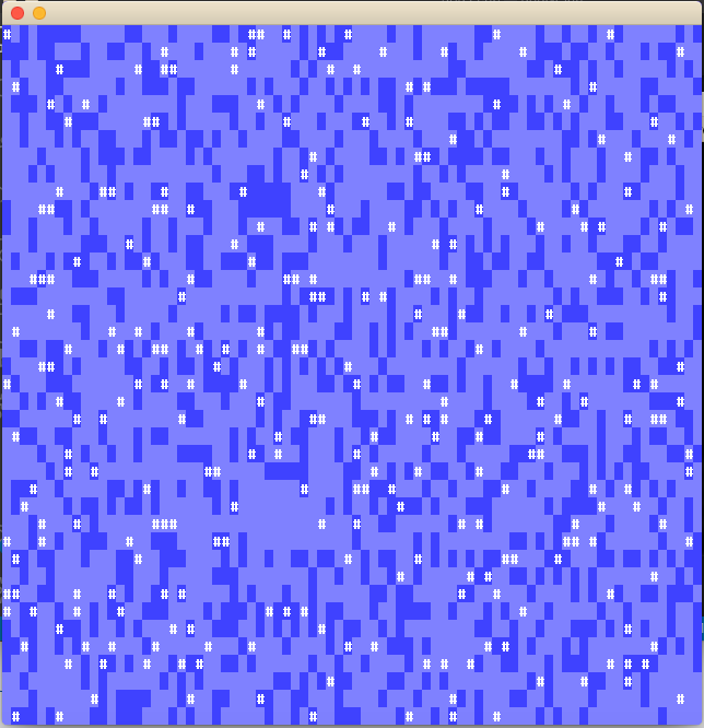
This will cause a window to open that looks something like this:

The white ‘#’ are blocking tiles that cannot be “stepped” on, the dark blue areas are tiles with edge costs that are higher to travel to than the light colored tiles. With out “maze” constructed, we can now start implementing the Path finding algorithms.
Path Finding Algorithms
There are many pathfinding algorithms that can be used for traversing this type of map. The simplest “maze solving” path finding algorithm is Depth First Search, which will find a path from a start node to a goal node if one exists, but it is not guaranteed to be a shortest path, nor does it take edge cost into consideration, so its not the “cheapest” path either. Depth First Search can be implemented either recursively or, by using a stack data structure to process iteratively.
The next step up is standard Breadth First Search, which WILL produce a shortest path with the caveat that it does not consider edge cost, so it is only a shortest path in terms of number of edges traversed. This is managed by the use of a FIFO Queue data structure.
The two best options for path finding in this case are Dijkstra’s algorithm which i have covered in previous articles in relation to general graphs, but not grids, and A* search. A* search is a heuristically guided adaptation of Dijkstra’s Algorithm, or put differently, Dijkstra’s Algorithm is a special case of A* where the value of the heuristic is 0.
What makes transforming a grid into an adjacency list graph is that because we have the spatial information from the grid, we can easily incorporate a manhattan distance based heuristic, which when added to the edge cost priority based search of dijkstra’s algorithm yields an efficient A* search algorithm.
Just as in Dijkstra we will be using a min-heap priority queue, and std::map to keep track of our path.
Because A* and dijkstra’s algorithm are so closesly related, a standard dijkstra implementation is a good place to start, and in truth, we only need to add less than five lines of code:
The heuristic function is at lines 10 through 17, It simply computes the manhattan distance from the current vertex to the goal vertex, and multiplies it by the lowest edge cost.
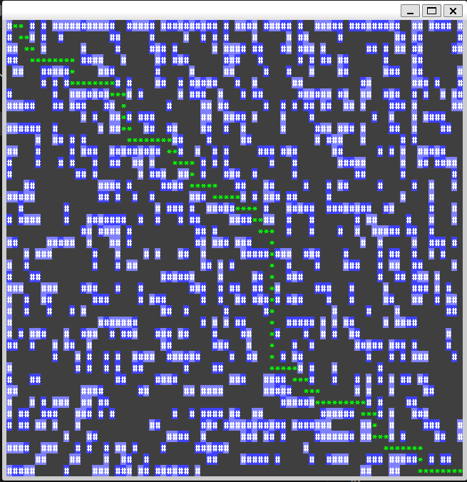
search() functions exactly the same as standard dijkstras algorithm, but when adding vertexes to the priority queue, the priority is new_cost + heuristic instead of soley new_cost. Thats the only Difference! but what a difference it is, as it reduces the number of nodes examined by a large margin. If you look at the inner loop of the A* algorithm, you can see that i color vertexes on the grid as they are examined, so that we can watch the search progress. Notice that it ignores blocked tiles completely (as all of our shortest path algorithms should), but that it also skips processing a large amount of the high cost tiles, as it favors lower cost tiles that have the shortest manhattan distance to the target.
Starting to explore:

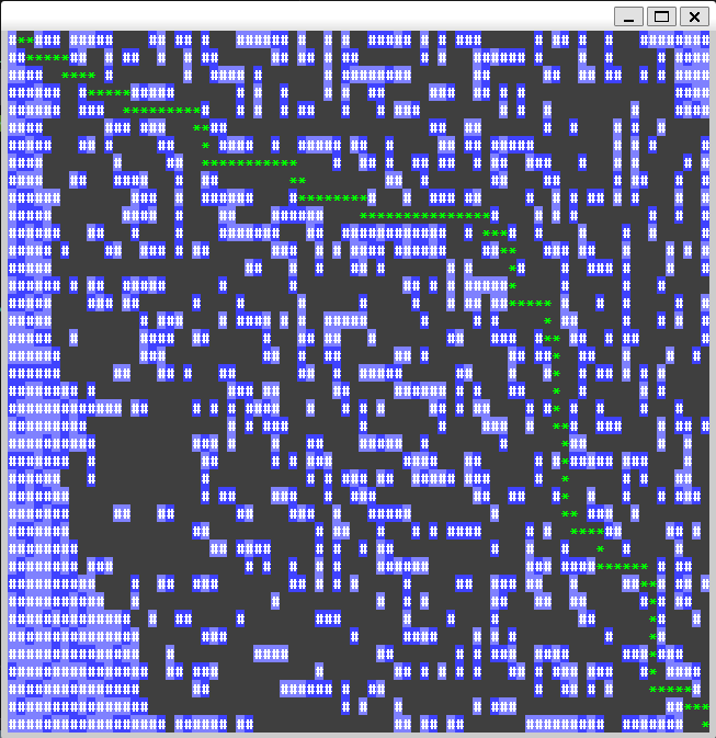
Progressing:

More:

More:

And Path Found!

Allright, well it definitely found a short path, but it is still exploring far too many nodes than we would like. So what should we do? The first step would be to try a different heuristic. How about using euclidean distance instead of manhattan distance?
    int heuristic(Graph& G, int u, int v)
    {
        node a = G.verts[u];
        node b = G.verts[v];
        int distx = abs(b.x - a.x);
        int disty = abs(b.y - a.y);
        distx *= distx;
        disty *= disty;
        int dist = sqrt(distx+disty);
        return dist;
    }
Lets see how we did:
Hmm. We’re still visiting an awful lot of nodes. Let’s try ratcheting up the heuristic by adding a delta value. A delta value is a number we multiply the distance by in the heuristic.
    int heuristic(Graph& G, int u, int v)
    {
        int delta = 5;
        node a = G.verts[u];
        node b = G.verts[v];
        int distx = abs(b.x - a.x);
        int disty = abs(b.y - a.y);
        distx *= distx;
        disty *= disty;
        int dist = sqrt(distx+disty);
        return delta * dist;
    }
Lets try 5:
Ok, now we’re trimming the search space! Let’s see what a delta of 15 gets us:
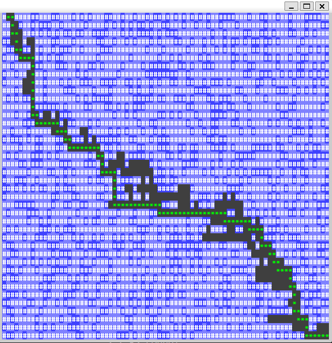
Wow! Clearly with a proprly tuned heuristic, A* is an amazingly efficient algorithm for trimming the search space. And there are many variants that can be adapted for all kinds of uses, as demonstrated here it can be used for path finding in video games very easily. It’s original use was for robotic AI path finding as part of the “Shakey” project at Stanford university. Regardless of what you use it for, I’m sure you will find it as cool and interesting as just about everybody else.
Full code for the implementation as shown here is available on my github at: