Memory Resident B+ Trees

Since Bayer & McCreight introduced the family of balanced search tree’s collectively known as “B Trees” in their 1972 paper[1], they have traditionally been used as a data structure for external storage devices, which is why they are very often used in implementing on-disk filesystems. Recent examples of filesystems using some form of B Tree are ReiserFS, btrfs, bcachefs, and even Microsoft’s NTFS, just to name a few. Another domain where B Tree’s are pervasive is in both relational and non relational databases. MySQL and PostgreSQL both provide B+ tree based indexing, for example.

The structure of the nodes make them particularly well suited for these kinds of tasks. Nodes in B Tree’s very have a very large fan out, leading to the trees themselves having a shallow depth. They are commonly described as “Bushy”, meaning values can be found in very few “probes”.

With the cost of memory experiencing a cost/performance curve reminiscent of what CPU’s have traditionally experienced, the non-optimal space usage of B Tree’s has become less of a limiting factor to their usefulness as in memory data structures. And people have been paying attention.

In 2013 Google released their opensource B Tree Map for C++ as a drop in replacement for the Red/Black Tree traditionally found in STL map implementations, as well as in the standard libraries of many popular programming languages. Bucking the trend alongside google, is the Rust programming language, which also makes use of a B Tree for the standard library Map and Set types.

B Trees vs. B+ Trees

According to CLRS[3], a B Tree is an ordered search tree who’s nodes contain between M/2 and M-1 keys, and M/2 and M children, and which has all of its leaf nodes at the same level which is the height of the tree. B Tree’s Are perfectly balanced and so perform all operations in O(log N).

The paper which originally presented B Tree’s listed several variations as possible optimizations. Two of those variants which have gained popularity are the B+ and B* trees. B+ Trees have become so popular that generally speaking, when people say “B Tree’s” they are usually referring to some form of B+ Tree.

So what exactly is a B+ tree, anyway? Well, it’s actually made up of (at least) two separate data structures. The index set is made up of a B Tree, and it is used to index the entry set. The entry set is a linked list of all the entry’s that the tree is used to efficiently navigate through. So in a quite literal sense, a B+ Tree is exactly that: a B Tree, Plus a linked list.

For the remainder of this post, when I say B Tree, I’m talking about B+ Tree’s except when specifically mentioned. B+ tree’s have several properties which offer advantages with regards to space usage and iteration compared to “traditional” B Tree’s, while simultaneously simplifying their implementation. B+ Tree’s uses it’s internal nodes as an index, to guide the search to the appropriate leaf node which stores a pointer to the actual data. Additionally, B+ Tree’s also link sibling nodes together in a linked list, which allows for fast in order iteration.

I have read many, many books on data structures and algorithms, and while B Tree’s are mentioned in practically single one of them, I have come across exactly one which includes a working example of B Tree insertion. In addition, each book describes them slightly differently. The most rigid definition of what constitutes a B Tree is thanks to Knuth(who else?). On the whole however, B Tree’s don’t have as nearly a rigid definition as AVL tree’s or Red/Black Tree’s, despite being more rigidly balanced. This leaves quite a bit of wiggle room and explains why everybody implements them a little differently.

Implementing B+ Trees

Choosing a layout

In computer science, a “tree” is a recursively defined object. Take for example a binary tree: A binary tree is a tree, whos individual nodes are them selves binary trees. Obviously such a definition holds for B Tree’s as well, and we could implement B Tree’s similar to how we would a binary search tree, with nodes laid out as follows:

const int M = 4;

template <class T, class T2>
struct BPNnode {
      T keys[M-1];
      T2 vals[M-1];
      int n;
      bool is_leaf;
      BPNode* children[M];
      BPNode* next;
      BPNode* prev;
};

This is very similar to the description provided in CLRS for B-Trees, and it will work, but using such a node layout creates much more work for ourselves. In the above example, we have three separate arrays of two different sizes, which makes inserting and removing keys/values/children from the tree much more complicated than it need be.

If we accept that one position in the key and value array may be “wasted” we can greatly simplify things by just make all three arrays the same size. If in addition we impose the restriction on our tree’s that M must be an even number of at least 4 we simultaneously simplify the logic for splitting node when an insertion causes an overflow. That lead’s us towards the following layout:

const int M = 4;

template <class T, class T2>
struct BPNode {
     T keys[M];
     T2 vals[M];
     BPNode *children[M];
     BPNode *next, *prev;
};

We can still do better. Since all three arrays are now the same size, and since the values in those arrays are related, we can create an object to represent the tuple<Key, Value, Pointer>, and our node well contain a single array of that object, as shown below:

const int M = 4;
 
template <class T, class T2>
struct BPNode;               //needs forward declaration for use in BPEntry

 
//Our node well hold one array of size M of this object 
//Instead of three arrays as in the example above
template <class T, class T2>
struct BPEntry {   
    T key;
    T2 value;
    BPNode<T,T2>* child;
};

//Our greatly simplified layout.
template <class T, class T2>
struct BPNode { 
     BPEntry<T,T2> page[M];  //key, value, child
     int n;                  //number of entries in this page
     BPNode *prev, *next;    //linked list pointers to siblings
};

In a B+ Tree the internal nodes don’t contain any data pointers, so our internal nodes will use the BPEntry’s “child” pointer to point down the tree towards the proper leaf, leaving the value field empty. Conversely, as leaf node’s in a B+ tree don’t have child pointers, they will use the value field, leaving the child pointer empty. In this way we handle the two “different” node types used for internal and leaf nodes.

By arranging our nodes in such a layout we have also serendipitously transformed each node of our B+ Tree to simultaneously be an ordered array based symbol table! This observation presents us with a decision: do we leave our nodes as Plain Old Data structures, or should we add a layer of abstraction, by implementing our B+ Tree nodes as “Pages”.

A Touch of Abstraction

By viewing each node as a page, it gives us greater flexibility with how we structure the nodes. So long as a data structure provides the methods listed below for BPNode, we can use any data structure we want. An ordered array is the standard. My first implementation was a “leaky” abstraction of pages, by using the C++ friend keyword. I’ve since cleaned it up by adding appropriate accessors to the BPNode API.

const int M = 4;
 
template <class T, class T2>
class BPNode;

template <class T, class T2>
struct BPEntry {   
    T key;
    T2 value;
    BPNode<T,T2>* child;
    BPEntry(T k, T2 v, BPNode<T,T2>* c) : key(k), value(v), child(c) { }
}; 

template <class T, class T2>
class BPNode {
    private:
        BPEntry<T,T2> page[M];
        int n;         // number of entries in page
        BPNode* next; // for efficient level  order 
        BPNode* prev; // traversal using O(1) extra space
        BPNode* split();       
    public:
        BPNode(int k = M);
        int size();
        bool isFull();  
        int floor(T key);
        int search(T key); 
        BPNode*  insertAt(BPEntry<T,T2> entry, int position);
        BPNode*  insert(BPEntry<T,T2> entry);
        BPNode* removeAt(int position); 
        BPEntry<T,T2>& at(int position);
        BPNode* leftSibling();
        BPNode* rightSibling();
        ~BPNode() {

        }
};

The interface for the node class is actually pretty straight forward. I’ll go through them all, giving extra attention where I feel it’s needed. The private members are our array of BPEntry structures, and the variable n, which is used to hold the number of entries currently in the node. The next/prev pointers are for pointing to the nodes siblings. These are used for efficient level order traversal, particularly of the leaf level, as this represents an in order traversal of the data stored in the tree. They are accessed through the leftSibling() and rightSibling() methods. The split() method is used during the insertion process, and I will explain more below.

The constructor is used for setting the initial entry count. The method size() returns the number of entries in the node, and isFull() is a quick test if the node has room for insertion or not.

template <class T, class T2>
int BPNode<T,T2>::size() const { 
     return n; 
}
 
template <class T, class T2>
bool BPNode<T,T2>::isFull() {
    return !(size() < M);
}

The next two methods are used for finding indexes in the page array. The method search(T key) searches for an exact match of the key, and if present returns its index in page[], upon failing it returns -1. The method floor(T key) is used for determining the position in page[] where an entry should be inserted.

template <class T, class T2>
int BPNode<T,T2>::search(T key) {
    for (int j = 0; j < n; j++)
        if (key == page[j].key)
            return j;
    return -1;
}

template <class T, class T2>
int floor(K key) {
    int j;
    for (j = 0; j < n; j++)
        if (j+1 == n || key < page[j+1].key)
            break;
    return j;
}

Despite maintaining an ordered array, AND despite that fact that B+ Trees themselves generalize a binary search of an ordered collection, it is actually more efficient to use a simple linear search as shown above, for all but the largest sizes of M when using B+ Tree’s as an in-memory data structure. If you want to use binary search instead, it will obviously work just fine, but do you really need to use binary search for 8 or even 16 elements?

Whichever search method you choose, now that we can obtain the index of entries, we can implement the logic to insert and remove values from those given positions, which is exactly what insertAt() and removeAt() do. This is one area where bundling everything into page elements really leads to a concise implementation. On side node, if you wish to implement top down tree’s for thread safety reasons, you’ll want to move the split-on-overflow portion of these methods out of these methods.

template <class T, class T2>
BPNode<T,T2>* BPNode<T,T2>::insertAt(BPEntry<T,T2> entry, int j) {
    for (int i = n; i > j; i--)
        page[i] = page[i-1];
    page[j] = entry;
    n++;
    if (isFull()) return split();
    else return nullptr; 
} 

 
template <class T, class T2>
BPNode<T,T2>* BPNode<T,T2>::removeAt(int j) {
    int i;
    for (i = j; i < n; i++)
        page[i] = page[i+1];
    n--;
    if (n == 0)
        return next;
    return this;
}

The removeAt(int) method is simple array deletion, that shuffles all of the elements to the right of the element being deleted over by one. If this causes the node to be come empty, the node replaces its self with its neighbors. I’ll go in to more detail on this when I cover deleting items from the B+ Tree.

Insert at places an entry at the provided position, moving all items over one space to make room for it. If an insertion does not cause a node to become full, we just return the node. If it does become full, we call the nodes split() method.

template <class T, class T2>
BPNode<T,T2>* BPNode<T,T2>::split() {
    BPNode* new_node = new BPNode<T,T2>(M/2);
    for (int i = 0; i < M/2; i++) {
        new_node->page[i] = page[M/2+i];
    }
    n = M/2;

    new_node->next = next;
    if (next != nullptr) 
        next->prev = new_node;
    next = new_node;
    new_node->prev = this;
    return new_node;
}

Split() allocates a new node, copies the rear half of the current nodes page[] array into the new node, and sets both nodes sizes to M/2. After that, the newly created node is hooked into it’s siblings as a linked list, and returned for inclusion in it’s parent.

BPNode* insert(bpentry& entry) {
       int j = n;
       while (j > 0 && page[j-1].key > entry.key) {
             page[j] = page[j - 1];
             j--;
       }
       page[j] = entry;
       n++;
       if (isFull()) return split();
       else return nullptr;
}

The insert() method above does not take an index argument, and instead places the item in its correct position with insertion sort. It might seem redundant to have two ways of inserting elements into the leaf, and indeed we could get away with one, but you’ll see why this is preferred when we cover insertion into the tree. Speaking of which, with these method’s in place we have what we need to begin implementing our B+ Tree, so let’s get to it.

Inserting Elements In B+ Tree

So far we’ve only talked about the individual nodes of the tree. Now it’s time to take a step back and look at the bigger picture. The most common use case for in-memory B+ Tree’s is for use as a dictionary, and such our B+ Tree should implement the basic Dictionary ADT API, mainly insert, get, search, and remove. I’ve also decided to add STL compatible Iterators so we can use C++’s foreach loops on our B+ Tree.

 
template <class T, class T2>
class BPTree {
    public:
        using iterator = BPIterator<T,T2>;
    private:
        using bpnode = BPNode<T,T2>;
        using nodeptr = bpnode*;
        nodeptr root;
        int height;
        int count;
        void printLevel(bpnode* node);
        void printNode(bpnode* node);
        bpnode* insert(bpnode* node, T k, T2 v, int ht);
        bpnode* erase(bpnode* node, T key, int ht);
        bpnode* splitRoot(bpnode* node, bpnode* new_node);
        bpnode* mergeNodes(bpnode* a, bpnode* b);
        bpnode* min(bpnode* node, int ht);
        bpnode* min(bpnode* node, int ht) const;
        iterator search(bpnode* node, T key, int ht);
        void cleanup(bpnode* node);
        T nullKey;   //for use in blank entries.
        T2 nullItem; // ^  ^
    public:
        BPTree();
        BPTree(const BPTree& o);
        ~BPTree();
        void insert(T key, T2 value);
        void erase(T key);
        iterator find(T key);
        T min();
        void sorted();
        void levelorder();
        iterator begin();
        iterator end();
        iterator begin() const;
        iterator end() const;
        BPTree& operator=(const BPTree& o);
};

I’ve introduced the full class definition, but this post will be primarily concerned with insertion and search, this post is already getting pretty long and deletion would make double it’s length. Remember when I said implementing those in-node methods was going to make implementing the tree it’s self much simpler? I wasn’t kidding. Let’s Take a look at implementing insertion.

Insertion begins by checking the level of the node we are currently processing. If we’re not at the bottom level, we find the correct child pointer for inserting our value into. Once we have reached the leaf level, we insert our new value into the leaf. If insertion causes an overflow the node calls it’s internal split method, returning the newly created node, who’s key is passed up to be inserted in the parent of the node it was split from.

template <class T, class T2>
void BPTree<T,T2>::insert(T key, T2 value) {
    nodeptr new_node = insert(root, key, value, height);
    if (new_node != nullptr) {
        root = splitRoot(root, new_node);
    }
} 
 
template <class T, class T2>
typename BPTree<T,T2>::bpnode* BPTree<T,T2>::insert(bpnode* node, T key, T2 bpnode* insert(bpnode* node, K key, V value, int ht) {
        int i, j;
        bpentry nent = bpentry(key, value, nullptr);
        if (ht == 0) {
            return node->insert(nent);
        } else {
           j = node->floor(key);
           bpnode* result = insert(node->at(j++).child, key, value, ht-1);
           if (result == nullptr) return nullptr;
           nent = bpentry(result->at(0).key, nullItem, result);
       }
      return node->insertAt(nent, j);
}

If at the root, the root is split, we call the splitRoot method, which is even simpler than the BPNode::split() method. It stores the current root in a temporary variable, ‘oldroot’, allocates a new root node of size 2, and points to the node returned by insertion, and the new root.

template <class T, class T2>
typename BPTree<T,T2>::bpnode* BPTree<T,T2>::splitRoot(bpnode* head, bpnode* new_node) {
    nodeptr oldroot = head;
    head = new bpnode(2);
    head->at(0) = BPEntry<T,T2>(oldroot->at(0).key, nullItem, oldroot);
    head->at(1) = BPEntry<T,T2>(new_node->at(0).key, nullItem, new_node);
    oldroot->next = new_node;
    HT++;
    return head;
}

Searching is even easier. Again, we track our position in the tree by using the height of the tree. While it may seem hackish compared to say, an isLead flag as seen in many implementations, it is also one less variable for each node to both store, and monitor. For return values, I prefer to use an iterator, as I’m a firm believer that the iterator pattern produces cleaner code. If you prefer, you could return a BPEntry object, an std::pair<T,T2> of key and value, or whatever else you feel like returning.

template <class T, class T2>
typename BPTree<T,T2>::iterator BPTree<T,T2>::find(T key) {
    return search(root, key, HT);
} 
 
template <class T, class T2>
typename BPTree<T,T2>::iterator BPTree<T,T2>::search(bpnode* node, T key, int ht) {
    int j = node->floor(key);
    if (ht == 0) {
        j = node->search(key);
        if (j > -1) return iterator(node, j);
        else return end();
    }
    return search(node->at(j).child, key, ht-1);
}

By keeping our nodes in a linked list with their siblings, a simple traversal of the leaf level will yield our keys in sorted order. We’ll come back to this property in a moment, as it makes implementing an iterator for our tree’s about as easy it gets.

template <class T, class T2>
void BPTree<T,T2>::sorted() {
    bpnode* x = min(root, HT);
    while (x != nullptr) {
        for (int j = 0; j < x->size(); j++)
            cout<<x->at(j).key<<" ";
        x = x->leftSibling();
    }
    cout<<endl;
}

template <class T, class T2>
typename BPTree<T,T2>::bpnode* BPTree<T,T2>::min(bpnode* node, int ht) {
    nodeptr x = root;
    while (ht-- > 0) {
        x = x->at(0).child;
    }
    return x;
}

Before I cover iterators, I want to show how we can also use the sibling lists to efficiently implement level order traversal of the tree without needing a queue.

 template <class T, class T2>
void BPTree<T,T2>::printNode(BPNode<T,T2>* node) {
    if (node != nullptr) {
        cout<<"(<";
        for (int j = 0; j < node->size()-1; j++)
            cout<<node->at(j).key<<", ";
        cout<<node->at(node->size()-1).key<<">) ";
    }
}

template <class T, class T2>
void BPTree<T,T2>::printLevel(BPNode<T,T2>* node) {
    if (node == nullptr) return;
    BPNode<T,T2>* x = node;
    cout<<"[ ";
    while (x != nullptr) {
        printNode(x);
        x = x->rightSibling();
    }
    cout<<"]"<<endl;
}

template <class T, class T2>
void BPTree<T,T2>::levelorder() {
    nodeptr x = root;
    int ht = HT;
    while (ht >= 0) {
        printLevel(x);
        x = x->at(0).child;
        ht--;
    }
}

Using the above code for level both level order traversal and inorder traversal, we can check that our B+ Tree is working. We’ll Insert the characters “A B T R E E E X A M P L E W I T H A L O T O F K E Y S” as the key, and their position in the above list of characters as the associated value. Once the tree is built, we’ll call sorted() and levelorder().

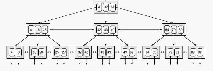
A A A B E E E E E F H I K L L M O O P R S T T T W X Y 
 [ (A | M) ]
 [ (A | E | I) (M | R) ]
 [ (A | A | E) (E | F) (I | L) (M | O) (R | T | W) ]
 [ (A | A) (A | B) (E | E) (E | E | E) (F | H) (I | K) (L | L) (M | O) (O | P) (R | S | T) (T | T) (W | X | Y) ]

That’s the tree built with M = 4, let’s see the effect of M = 8:

A A A B E E E E E F H I K L L M O O P R S T T T W X Y 
 [ (A | E | L | P | T) ]
 [ (A | A | A | B | E | E) (E | E | E | F | H | I | K) (L | L | M | O | O) (P | R | S | T | T) (T | W | X | Y) ]

As you can see, if with a fan out of 8, the tree has only 2 levels. Searching in B+ Tree’s is obviously fast. In addition to being examples of balanced ordered search tree’s, and there nodes examples of ordered array key value maps, the leaf level of of B+ Tree’s are an example of an ordered, unrolled linked list! Talk about a hodge podge of data structures.

I think this is probably a good place to stop for today, In my next post ill be covering deletion, and implementing iterators for B+ Trees. Until next time, Happy Hacking!

B Trees vs. B+ Trees

Implementing B+ Trees

Choosing a layout

A Touch of Abstraction

Inserting Elements In B+ Tree

Further Reading

max

Recent Posts

Archives

Meta

Kruskal’s Minimum Spanning Tree Algorithm

Conway’s Game Of Life

The Shunting Yard Algorithm: Simple Bottom-up Expression Parsing

From Parse Trees To AST’s: Predictive Parsing using Recursive Descent