
In part one of my article on open address hash tables i discuss hash functions, initializing the table and buckets, as well as insertion and searching via linear probing.

Hash Tables
Hash tables are a fantastic alternative to binary search trees when it comes to simply implementing an associative array or set, often times offering O(1) insert, search, and removal times in contrast to the O(log N) performance of a balanced tree, and their implementation is leaps and bounds easier than say, a red black tree.
If maintaining sorted order is not a critical property for your data, hash tables are the way to go. While binary search trees use comparison for finding positions in the tree, hash tables work by computing a key, using certain properties of the keys themselves to compute an array index. A downside to this approach is that this can result in whats called collisions, or a “hash crash” when two or more keys map to the same array index, in which case a collision resolution strategy is needed. Two of the more popular methods for dealing with key collisions are separate chaining, which i’ve covered previously, and open addressing which i will be covering in this article.
From keys to Indexes
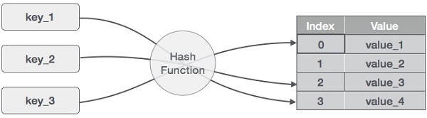
As i mentioned in the introduction, hash tables work by transforming a key into an array index. For the sake of simplicity i will be assuming that the keys we are hashing are strings. There are numerous hash functions floating around and all of them have their associated pros and cons. Ideally, a hash function should be chosen that spreads keys out evenly amongst table slots and will result in the minimum amount of collisions as possible. The hash function i will be using in this example is called “cyclic shift hashing”:
An array by any other name
A hash table at its most basic is an array. Because we are storing our key with our value in our hash table, we need to create a data structure for our table items, or “buckets”:
While the hash table its self is centered around the array of buckets, there is also satellite data that goes with it to become the “hash table” it was born to be, so its nice to wrap all this data together into its own structure. The satellte data that we need to track is the number of items currently being held in the hash table, which we call “count” and the number of buckets the table holds, which we call “tableSize”:
With those pieces in place we have set the foundation for hash table, and if we had a “perfect” hash function that could 100% avoid collisions our job would be essentially done. But as we know, the second half of building a hash table is handling collision resolution.
Handling the Hash Crash
The method for collision resolution that i will be employing in this article is called linear probing, its self a generalization of whats called “open addressing”. What happens is once we calculate the index of the bucket to plays our key/value pair in, we check if it is already populated. If it is not, we simply place our item in that bucket and were done. If our hash collides with another item already residing in that bucket however, we check the next bucket up, and so on, until we find a free slot:
Now, the “Table Full” error is a stop gap measure, and something we should work to actively avoid. And should only be used as a last resort in environments with sever memory constraints.
A brief aside on dynamically sized hashed tables
As mentioned above, we strive to avoid running out of space in our hash table. In practice, a hash tables performance is married to its load factor, that is, the number of occupied buckets versus total available buckets. As this value approaches 1 the performance of our table degrades from initially O(1) (or damn close to it) to practically O(n) and worse: insertion failure. Thus we monitor our tables load factor, and when it crests a predetermined value, usually 0.5 – 0.7, we would rebuild the table by allocating a new table of twice the current size, and re hash all of our items into the new table. But thats a subject for another article.
Data Retrieval
An associative array certainly would not be much good if once data was inserted it was lost to us. Thus, once we’ve added an item to our hash table, we need a convenient way of retrieving it, and this is one area where the simplicity of linear probing really shines, in fact, we pretty much already covered the “how-to” of this operation during insert! The process works as follows: we compute the hash of the key were searching for and check the bucket the key indexes to. If the item in that bucket matches the key (and not just hash!) we return the associated value, if it doesn’t, we search each following bucket for a matching key or until we hit a NULL value, which would indicate a search failure.
Stay Tuned!
Thats it for this article, but come back for part two, where i’ll discuss another collision resolution strategy: seperate chaning.
-max